
Applying Dynamical Analysis to Human-Environment Interactions
Background
MY research (and many others’) is fueled by the idea, how to humans affect the environment, and vice versa? We like to think that human societies attempt to alter environment cycles to improve both ecosystem productivity and quality, but I feel like it is usually just that first one. This begs the question, can these coupled human-environmental systems be modeled? My final project for my Ecohydrology course was a simple exploration into a very specific mathematical model, proposed in Poporato et al. (2015).
The model proposed here is a nonlinear system of two ordinary differential equations. This type of system lends itself well to a simple dynamical analysis, an excellent tools that provides insight on interactions and feedbacks between two variables and their parameters. This small project offers an exploration into this pre-proposed mathematical models.
Analysis
The model in the paper is given by the two nonlinear ODEs:
\[\begin{align*} \frac{\text{d}q}{\text{d}t} &= \eta_0 + k_{nat}q(A-A_{ag}) - k_{ag}A_{ag}-c\bigg(\frac{q}{q_0}\bigg)^{\alpha} \\ \frac{\text{d}A_{ag}}{\text{d}t} &= (k_h q A_{ag} + A_0)\bigg(1-\frac{A_{ag}}{A}\bigg) \end{align*}\]where \(q\) and \(A_{ag}\) are the two main variables in this system, representing ecosystem quality and agricultural land area, respectfully. All other variables are constants that can be changed depending on the ecosystem. \(q_0\) is some reference ecosystem quality, \(A\) is the total land area, which is the sum of \(A_{ag}\) and \(A_{nat}\), the natural land area. \(A_0\) is the rate of external market influence and \(\eta_0\) are external inputs from surroundings. Finally, there are control parameters that also differ based on the ecosystem and how much human influence there is. \(k_{nat}\) is a conversion from quality to ecosystem services, \(k_{ag}\) is the degradation rate from nearby agricultural practices, and \(k_h\) is the development rate of agricultural land in response to production. Lastly, two other parameters are defined, \(c\) is the rate of turnover and \(\alpha\) is some equilibrium control value. Quite a mouthful to define all parameters of this system, but it shows how important many different human-environment processes are to the well-being of an ecosystem.
An analytical solution to this system is highly improbable due to the nonlinear nature of the system. Therefore, we hope to approximate the phase portrait near a fixed point \((x^{*},y^{*})\). Figure 3 in Poporato et al. (2015) has already identified a fixed stable point at \((q,A_{ag})=(0,0.5)\). Thus to linearize the system, we evaluate the Jacobian matrix at this fixed point, resulting in
\[\begin{bmatrix} k_{nat}\bigg(A-\frac{1}{2}\bigg) & -k_{ag} \\ k_h\frac{2A-1}{4A} & -\frac{A_0}{A} \end{bmatrix}\]To determine how this system behaves around this fixed point, we want to analyze the eigenvalues. We are interested in complex eigenvalues, because the system is classified as stable and behaves as a spiral/center. The eigenvalues are complex in this linearized system when the discriminant \(\tau^2 - 4\Delta<0\) (where \(\tau\) is the trace and \(\Delta\) is the determinant). Solving for this case, we find that the criteria for a stable linearized system is
\[\begin{equation} k_h > \frac{1}{k_{ag}}\bigg[ \frac{A_0^2}{A(2A-1)}-3A_0 k_{nat}+\frac{A(2A-1)}{4}k_{nat}^2 \bigg]\,. \end{equation}\]We will call the RHS of the above equation \(K(A_0,k_ag,k_{nat})\). What’s left to do here is an analysis. There are many ways to go about analyzing this equation - what I’ve decided to do is see how the math relates to the definitions of the variables.
Recall that a stable/spiral solution to this system corresponds to some equilibrium cycle. An unstable solution corresponds to the breaking of this cycle, for example mass degradation. So, assuming a fixed total land area \(A\), how does varying the parameters \(A_0\), \(k_{nat}\), and \(k_{ag}\) control this systems ability to behave as said limit cycle that oscillates between production and degradation? And does it make sense physically?
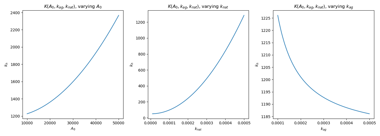
In the above figure, the three parameters \(A_0\), \(k_{nat}\), and \(k_{ag}\) are varied separately, and the relation \(k_h = K(A_0,k_ag,k_{nat})\) is plotted. Above this line, the discriminant is negative, the eigenvalues are complex, and the system exhibits a stable/spiral solution. In the first plot, as \(A_0\) increases, then the threshold for \(k_h>K(A_0,k_ag,k_{nat})\) to be true increases. This is physically interpreted as an increase in external markets driving land cultivation must be matched by the rate at which agricultural land is developed. For the center plot, using the same reasoning, we conclude that as we acquire more services from an ecosystem, then the rate at which agricultural land is developed must also increase. Again, this makes sense because more agricultural land provides more services. Finally, for the third plot, it is clear that as the degradation rate of a system increase (due to increased nearby agricultural practices), then the rate at which agricultural land is developed decreases. This may not be as obvious as the other two, but I am interpreting this as if humans take more than what they need (and therefore degrade an ecosystem), then eventually agricultural land will not be able to provide for humans. To me this sounds a bit like the !(tragedy of the commons)[https://en.wikipedia.org/wiki/Tragedy_of_the_commons].
The above statements may seem obvious and surface-level, but the analysis here showed that using a mathematical model allowed us to come to these conclusions. There are many different ways one can analyze the system of equations that I started with, but this is the route that I took. I hope you enjoyed this little foray into some mathematical modeling and dynamical analysis that I don’t often get to experience in my work.
References and Further Reading
- Modeling Human Decisions in Coupled Human and Natural Systems: Review of Agent-Based Models
- Excessive Rainfall Leads to Maize Yield Loss of a Comparable Magnitude to Extreme Drought in the United States
- Ecohydrological Modeling in Agroecosystems: Examples and Challenges
- Physical and Biological Feedbacks of Deforestation
- Catastrophic Shifts in Ecosystems